On the performance of D sets

If I google “dlang sets”, the first result is this forum post, “How to use sets in D?”. The main alternatives, brought up in the replies, consist of using std.container.rbtree or making a custom wrapper around the built-in associative arrays (AAs). I’ll explore and compare the performance of those options, then try to come up with something better and, more importantly, something that works in DasBetterC mode.

Experimental Setup

I’ve written four small parameterized benchmarks, one for each relevant operation on a mutable set data type:

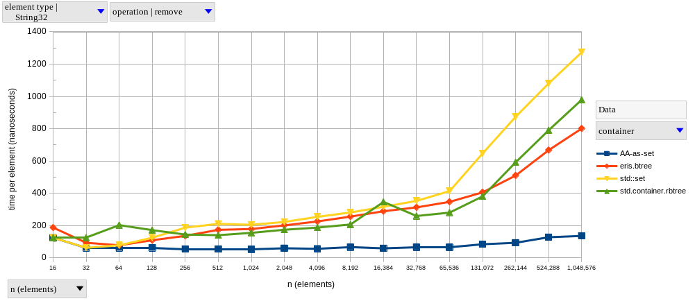
• upsert: creates an empty set container and upserts \(n\) random elements (of a given element type), measuring elapsed CPU time of all \(n\) insertions.
• lookupFind: inserts \(n\) random elements, then looks up these same elements in the set (checking that they were found), while measuring only the lookups.
• lookupFail: inserts \(2n\) random elements, removes the first \(n\), then looks them up (checking that they were NOT found).
• remove: inserts \(n\) random elements, then removes them one by one, measuring only removals.

In each of these, we measure elapsed CPU time (using clock) of performing all \(n\) operations. Then, we repeat that 30 times in order to eliminate some measurement noise. All elements are randomized once (using rand), in the very beginning of the test, with a fixed random seed, and the D garbage collector (GC) is executed before each of those repetitions. Finally, we vary \(n\) across powers of two, \(2^{4} \le n \le 2^{20}\).

Since the payload does not change while repeating each experiment, we estimate performance using Chen and Revel’s model: if \(measuredTime = realTime + randomDelay\), and \(randomDelay\) is always non-negative (the system can become slower at times due to other processes running, but not randomly faster), then the minimum value we can obtain of \(measureTime\) should be the best estimate of \(realTime\). Once we have the estimate of how long it takes to perform an operation \(n\) times, we’ll report that time normalized by the number of repetitions, that is, \(estimateTime(n) \div n\).

AAs and std.container.rbtree both lack support for custom allocators, which makes it really hard to precisely measure their memory usage. I’m aware of core.memory.GC, but it didn’t work as expected when I tried it and it could never be as precise as a custom allocator anyhow. Since I’m lazy, I chose to use GNU time’s report of resident set size (RSS) as a single way to measure memory usage across D, C and C++ programs.

GNU time can be used to report the maximum RSS of a program, and in each experiment that should correspond to the point in lookupFail after inserting \(2n\) elements. Then, we could get a (very rough) estimate of memory usage per element by dividing that value by the number of elements in each set. It should be noted, however, that these \(2n\) elements were generated at random and are being deduplicated by the set, so the birthday problem applies more and more as \(n\) grows. Therefore, we also need to record the maximum number of elements stored in the set during a program run. We also note that, for small \(n\), we expect max RSS to be incredibly imprecise, since most of it is being used by the language runtime.

For the sake of completeness, here’s more information about the system these micro-benchmarks ran on:

Host: Dell Inspiron 7559 (Notebook)
CPU: Intel i7-6700HQ (8) @ 3.500GHz
Caches (L1d, L1i, L2, L3): 128 KiB, 128 KiB, 1 MiB, 6 MiB
Memory: 16 GiB
OS: Pop!_OS 22.04 LTS x86_64
Kernel: Linux 6.2.6-76060206-generic
D compiler: ldc2 1.32.2
D flags: -O -release -inline -boundscheck=off
C++ compiler: g++ (Ubuntu 11.3.0-1ubuntu1~22.04.1) 11.3.0
C++ flags: -std=c++17 -O3
time: time (GNU Time) UNKNOWN
Shell: bash 5.1.16

And here’s a table with raw experimental results.

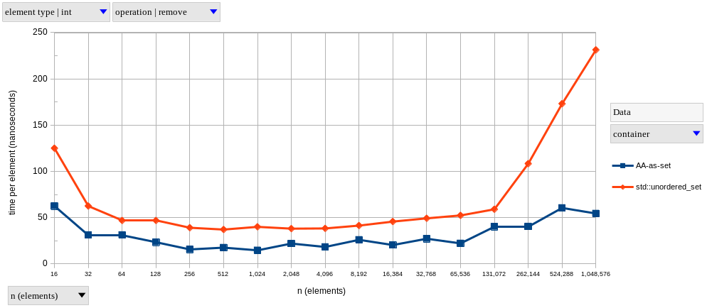
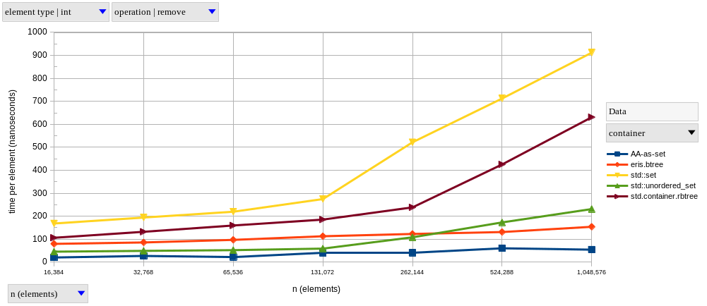
AA-as-set vs std.container.rbtree

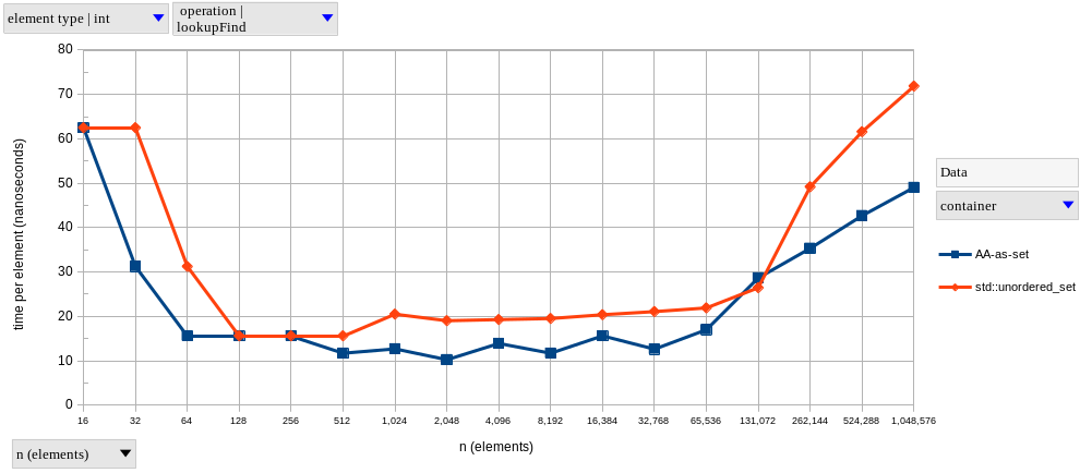
If we limit ourselves to the D runtime and standard library, we’ll be comparing hash-tables (AAs) and red-black trees (std.container.rbtree). Since our inputs follow a uniform distribution, their hashes ought to be uniformly distributed as well, which is pretty much the ideal situation for hash tables. Therefore, I expect the AA-based set to have much faster (average \(\mathcal{O}(1)\)) lookups than the tree-based set (\(\Theta(log_2 n)\)), and for lookup time to dominate other operations as well.

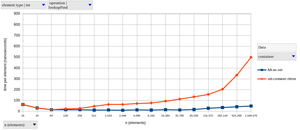
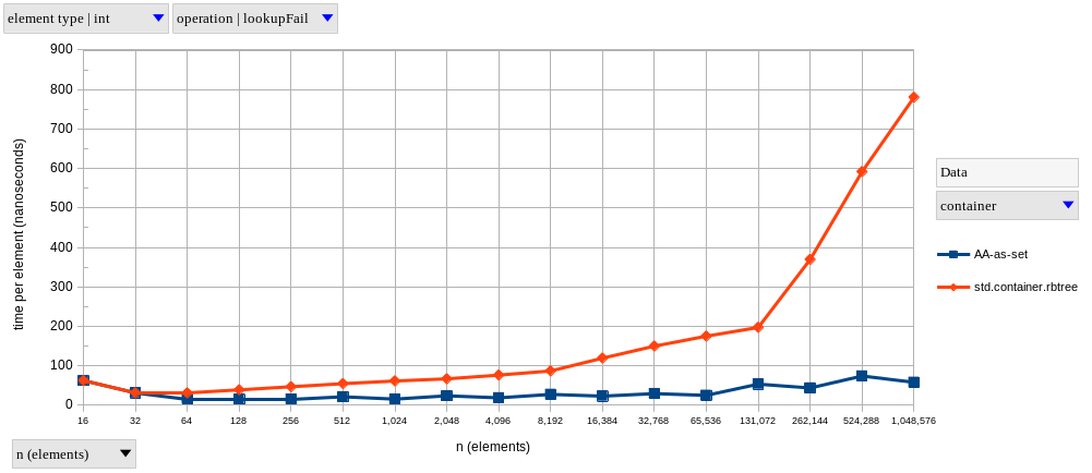
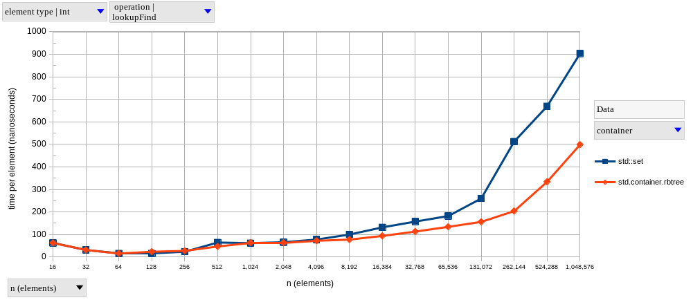
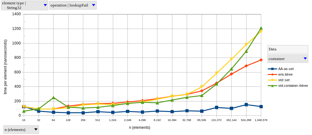
The two graphs above show results for lookupFind and lookupFail, respectively, using integer elements. As predicted, AAs exhibit near-constant time complexity. Meanwhile, lookups on the tree-based set become logarithmically slower as \(n\) increases – it only looks linear in our graphs because of the logarithmic scale on the horizontal axis.

The graph of our tree-based set looks like two connected lines, with the second having a larger slope. I’m guessing this happens because, after a certain point, we’re hitting the next level of the memory hierarchy much more frequently. Why do I think this? Well, my CPU’s L1d, L2 and L3 sizes are 128 KiB, 1 MiB and 6 MiB, respectively. Therefore, if we were to completely fill my L2 cache with 4-byte integers, it would fit at most \(262,144\) elements. Since our data structures are never as memory-efficient as a giant array with contiguous elements, we start hitting L3 a little earlier than \(n = 262,144\), and we see that that’s approximately where the slope changes.

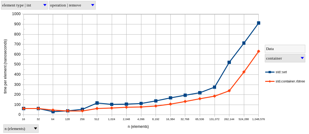
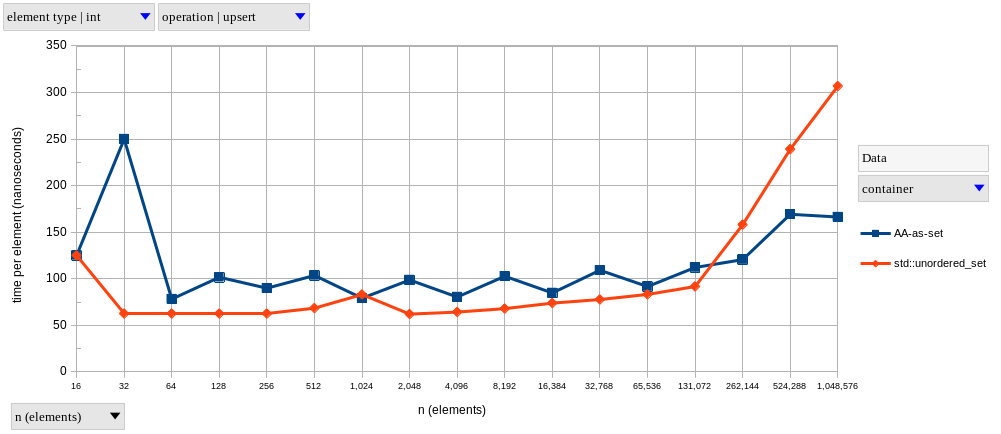
I won’t bother showing graphs for the other operations, since their shapes are pretty much the same. In fact, I’m only showing both lookupFind and lookupFail (and in the same vertical scale) to note that the difference between a successful and a non-successful lookup is much more significant in a tree-based set (find is 1.56x faster than fail at \(n = 2^{20}\)) than in a hash-based set (resp. 1.18x). Here’s a table summarizing the relative perfomance of these sets at a few input sizes:

Operation	AA speedup at \(n = 2^{7}\)	\(n = 2^{10}\)	\(n = 2^{20}\)
upsert	0.92x	1.74x	3.53x
lookupFind	1.50x	5.00x	10.17x
lookupFail	2.50x	3.94x	13.43x
remove	1.67x	4.60x	11.60x

It’s pretty clear that using AAs instead of std.container.rbtree should be preferred whenever you don’t need in-order iteration over set elements, as the performance gains range from pretty small to an order of magnitude (on most operations). That is, of course, if you can get a uniform distribution of hashes.

For memory results, see the next section.

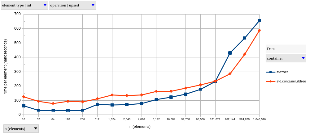
D vs C++

Some people consider D to be a successor to C++, so I’m also interested in comparing the set data structures in each language’s standard libraries. So, after some messing around with C++’s terrible templates and macros, I’ve ported our micro-benchmark program in order to add std::set and std::unordered_set to our comparison.

Before running anything, my expectations were that performance differences would come mainly from the different allocation strategies: garbage collection in D versus manual (de)allocations in C++. In particular, I expected D sets to have slightly faster removals due to the GC-deferred deallocations. I would normally expect allocations to be faster in C++ on average, but because the D GC is being executed before each round of operations, it shouldn’t affect upserts that much. I also expected memory usage to be higher in D, mainly due to its heavier runtime.

Since tree-based and hash-based sets have quite a big performance gap in these benchmarks, we’ll separate these two groups. With that said, let’s start with the tree-based containers, std.container.rbtree and std::set (charts below). Both have very similar performance (which is to be expected, since they’re both red-black trees), but the D version is usually a bit faster at larger \(n\). I was a bit surprised by the performance of upserts, which are faster in the C++ version for sets with less than a hundred thousand elements. This might be related to the performance of memory allocation with the D GC, as opposed to C++’s new.

Our hash-based set comparison went similarly, with the D version being slightly faster on lookups, but slightly slower on insertions. There was a bigger difference in removal performance in this group, with D AAs being consistently faster than std::unordered_set. Removal speedups range from ~1.5x, up to 4.25x for bigger sets. Once again, this might be explained by the different deallocation strategies; after all, D memory is only actually being deallocated during GC cycles, which either happen on insertions, or before the next experiment repetition (a manually-triggered full GC cycle which is not measured).

As for memory usage, here’s how our sets compare (graph below, but note the logarithmic scale on the vertical axis this time). Once again, we’re normalizing our estimate of memory usage by the number of elements in each set. As expected of our chosen memory metric (maximum process RSS), this leads to a huge overstatement of how much each element actually takes, at least for small \(n\). Therefore, this measurement is better interpreted as “what is the maximum amount of bytes each element could be taking, assuming nothing else in the entire program contributed to RSS”. For larger \(n\), however, I expect this estimate to tend towards the real per-element memory usage.

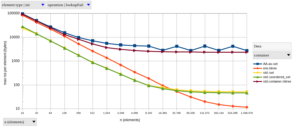
Assuming the measure for our largest \(n\) is the better estimate, we end up with the following:

container	max RSS per element (bytes)
AA-as-set	2759 B
std.container.rbtree	2371 B
std::set	51 B
std::unordered_set	46 B
eris.btree	12 B

While final values for the C++ containers seem reasonable, that’s far from true for the D sets. I expected D’s heavier runtime to inflate memory usage measurements, and we can see that in the left part of the graph as a roughly constant offset between the logarithmic curves of D and C++ containers. As we increased \(n\), the C++ programs started to converge towards something close to the true memory usage per element, but the D ones kept to a maximum RSS two orders of magnitude higher. Remember that max RSS stands for the greatest amount of physical memory the process occupied during its entire execution. Since both AAs and std.container.rbtree make heavy use of the GC, I assume that is what’s keeping the RSS high; perhaps it keeps freed memory around in order to reuse it later, instead of giving it back to the operating system.

Something you might notice in the last chart is that it includes memory usage for another set container, eris.btree. That’s my custom B-tree, which is implemented in D, but uses a custom allocator (based on malloc and free) instead of the D GC. We can see that, despite being implemented in D (and being run with the same heavier runtime), this data structure has similar behaviour to the C++ ones with respect to our measure of memory usage, beating them by approximately 4x at \(n = 2^{20}\). This also strenghtens the argument that the huge max RSS per element, obtained when benchmarking the D containers, is due to their usage of the GC and probably not even close to true memory usage (if only they supported custom allocators …).

The next section compares my custom eris.btree container with the other sets we’ve seen so far.

B-Tree Container

While D’s standard set containers have roughly equivalent (often slightly better) performance compared to their C++ counterparts, it turns out that C++ standard set containers are not actually that good to begin with. From what I could gather, these standard containers can’t be the fastest possible data types due to requirements of reference and iterator stability across mutating operations on the containers, as well as a few requirements related to const-correctness. This means that std::set (like std::map) pretty much has to be implemented with a binary tree (a red-black tree, to be more precise), and that std::unordered_set (like std::unordered_map) can’t use closed hashing (i.e. their hash table implementation has to use separate chaining). All of these restrictions lead to worse performance, mainly through less-than-optimal cache usage.

As far as I know, relational databases rely on B+ and B-trees because these data structures provide increased data locality on each node and, due to a fan-out that’s much higher than a binary tree, less pointer chasing when going down the tree. While these factors are especially relevant for data structures using hard disks as their underlying storage, they also apply to in-memory data strucutres. Therefore, I figured that a simple B-tree-based set would provide a good contestant against D and C++ standard containers. Let’s check the results:

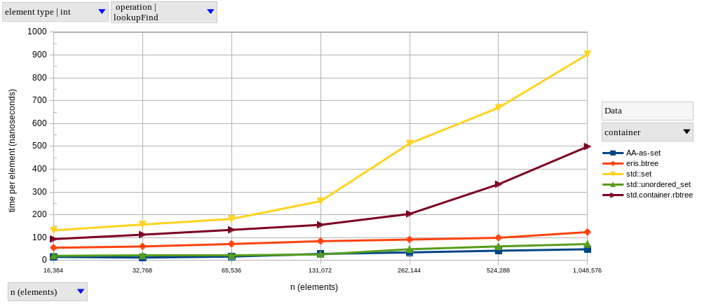
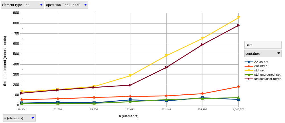
As we can see, for \(2^{14} \le n \le 2^{20}\), the performance of our B-tree is closer to hash-based sets than tree-based ones. B-tree operations have a theoretical time complexity of \(\Theta(log_m n)\), for some constant \(m \gt 2\); as \(m\) (the order of the B-tree) increases, this becomes “effectively \(\mathcal{O}(1)\)” for any real-world \(n\), which is precisely what we’re observing in these results. If you prefer relative speedups, here’s how our B-tree compares to other sets at \(n = 2^{20}\):

container / operation	upsert	lookupFind	lookupFail	remove
AA-as-set	1.09x	0.40x	0.32x	0.35x
std::set	4.31x	7.27x	4.70x	5.93x
std::unordered_set	2.02x	0.58x	0.42x	1.50x
std.container.rbtree	3.86x	4.02x	4.29x	4.10x

Looking at just the tree-based containers, we can see speedups of approximately 4x (and up to ~7x) across the board by using our custom B-tree-based set. In most cases, we still fall behind the hash-based containers, albeit by less than the order-of-magnitude margin they had over the red-black trees. The exception here is upsert, where the B-tree gets a little faster than the hash tables. As for memory, we covered that in the previous section already.

A B-tree’s main disadvantage is the fact that mutating operations may need to move multiple elements around in memory. This invalidates iterators and references to internally-held elements, but may also decrease performance for bigger elements.

Bigger Elements

A big part of “modern C++” is copy elision and move semantics. These features are supposed to interact nicely with RAII, and improve performance by avoiding unnecessary copies. While D also has some features to avoid copies, there’s definitely much less of a focus in that. Therefore, it should be interesting to compare our sets with bigger element types. In our case, we’ll use fixed-size arrays, each with exactly 32 bytes; they’re ordered by strncmp and hashed by a 32-bit FNV-1a function (in the previous experiments, we were relying on each language’s built-in ordering and hashing functions for integers).

In these benchmarks, I expected cache locality to play a smaller role, since fewer elements can fit in the cache now – our B-tree probably won’t get the same speedups it did before. To my surprise, the performance of C++’s std::unordered_set completely broke down with this bigger element type, to the point where I gave up on measuring its performance for any \(n > 10,000\). I’m not sure what’s happening, but std::unordered_set behaves linearly when holding elements with 24+ bytes, and this is reproducible with clang as well.

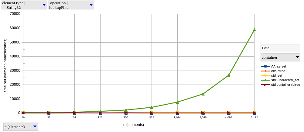
After removing the problematic std::unordered_set<String32>, our results (disappointingly) match my expectations, with the performance of eris.btree falling behind the AA implementation, and getting closer to (albeit still faster than) the other tree-based sets.

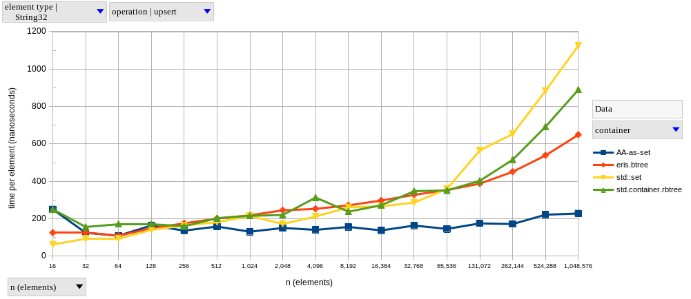
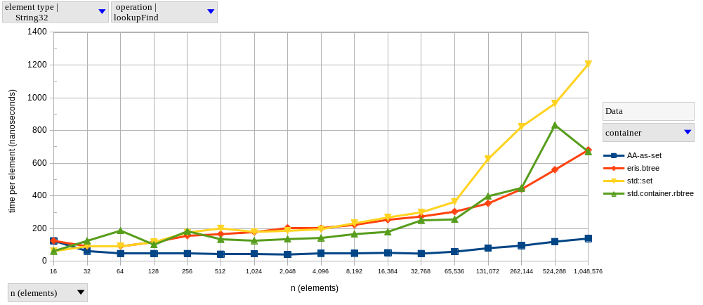
Here’s another speedup table for our B-tree at \(n = 2^{20}\):

container / operation	upsert	lookupFind	lookupFail	remove
AA-as-set	0.35x	0.20x	0.16x	0.17x
std::set	1.73x	1.77x	1.51x	1.59x
std.container.rbtree	1.37x	0.98x	1.57x	1.22x

Checking Assumptions

As I explained previously, I’m estimating time by picking the minimum measurement across 30 repetitions of each experiment. This might be surprising for some of you, who would have expected a report of average timing instead. I did some research on benchmarking techniques, and professional teams seem to prefer percentiles when measuring application performance. This is because most benchmark results don’t actually follow normal distributions, where mean and standard deviation would do the job.

Since we already have the data for that, we can perform a simple normality test to check whether we should have used the mean instead. For each of our parameterized experiments, we collect minimum, maximum, mean and the standard deviation of our 30 measurements. With these, we can compute the z-score of our extrema, and compare that to the 68-95-99.7 (a.k.a the \(1\sigma-2\sigma-3\sigma\)) rule.

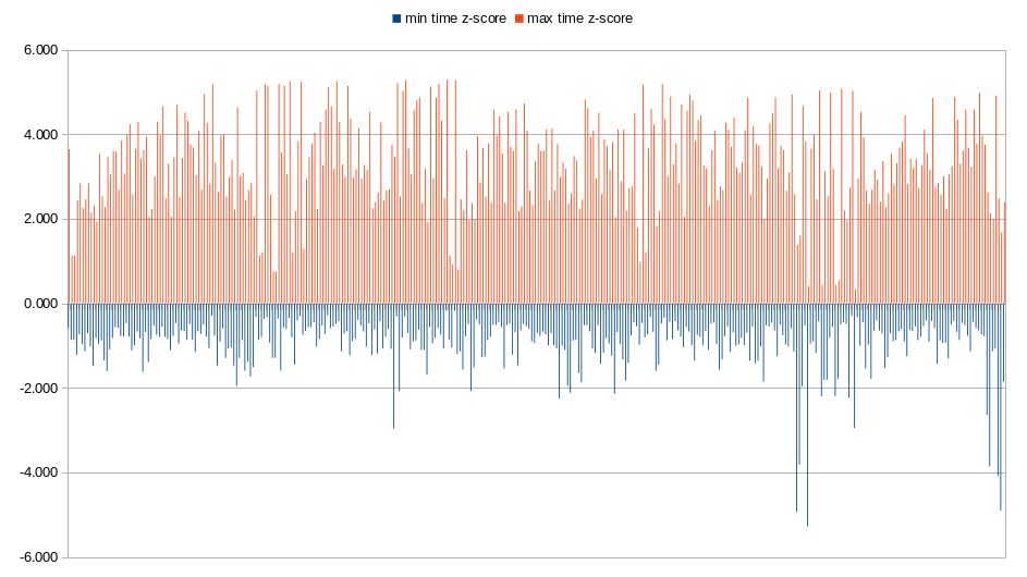
As we can see, there are many \(3\sigma\) (and even \(4\sigma\)) events in our maximum measurements. These imply that modeling our performance with a normal distribution would lead us to underestimate how much deviation there really is in our measurements. At that point, average elapsed time is not as meaningful, and, since I’m lazy, I didn’t want to implement a more advanced statistics collector.

What’s Next

For now, I’m satisfied with the performance my custom B-tree set was able to achieve. My next step is probably going to be improving its API before making it open-source.

As for further benchmarks, we could try exploring other payloads. Due to the uniform distribution of our inputs, hash sets have the upper hand. It would be interesting to test how well that performance stands up to less-than-ideal hash distributions.

At some point, I’ll also try to make a faster hash table in D (and make it -betterC compatible, of course). When I do, I’ll add it to these benchmarks as well, and maybe the next time I’ll be using the P50 percentile (the median), since now I have an efficient ordered set data structure which I can use to compute percentiles: eris.btree.